R

rstan

The rstan package is the workhorse, and the other packages mentioned in following rely on it or assume similarities to it. In general though, rstan is what you will use when you write Stan code directly. The following demonstrates how.

dataList =  list(X=mymatrix, y=mytarget, N=1000, K=ncol(mymatrix))

library(rstan)

modResults = stan(mystancode, data=dataList, iter=2000, warmup=1000)

model_debug = stan(mystancode, data=dataList, iter=10, chains=1)

mystanmodel = stan(mystancode, data=dataList, fit = model_debug, 
                   iter=2000, warmup=1000, thin=1, chains=4, cores=4)

print(mystanmodel, pars=c('Intercept', 'beta_1', 'sigma', 'Rsq'), probs = c(.05,.95), digits=3)

Inference for Stan model: 34b5bc624f3e17e6f88e764a5bc0c898.
4 chains, each with iter=2000; warmup=1000; thin=1; 
post-warmup draws per chain=1000, total post-warmup draws=4000.

           mean se_mean    sd     5%   95% n_eff  Rhat
Intercept 1.267   0.002 0.085  1.126 1.403  1396 1.004
beta_1    0.081   0.004 0.148 -0.157 0.331  1606 1.003
sigma     0.969   0.001 0.030  0.922 1.019  2313 0.999
Rsq       0.646   0.000 0.001  0.644 0.648  1816 1.002

Samples were drawn using NUTS(diag_e) at Wed Nov 09 15:32:08 2016.
For each parameter, n_eff is a crude measure of effective sample size,
and Rhat is the potential scale reduction factor on split chains (at 
convergence, Rhat=1).

library(shinystan)
launch_shiny(mystanmodel)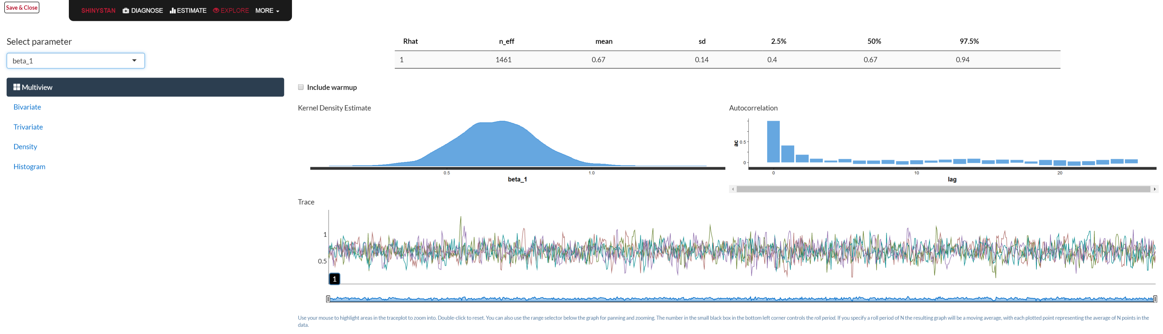

rstanarm

The rstanarm is a package from the Stan developers that allows you to specify models in the standard R format⊕The ‘arm’ in rstanarm is for ‘applied regression and multilevel modeling’, which is NOT the title of Gelman’s book no matter what he says.. While this is very limiting, it definitely covers a lot of the usual statistical ground. As such, it enables you to be a Bayesian for any of the very common glm settings, including mixed and additive models.

Key modeling functions include:

• stan_lm: as with lm
• stan_glm: as with glm
• stan_glmer: generalized linear mixed models
• stan_gamm4: generalized additive mixed models
• stan_polr: ordinal regression models

Other functions allow the ability to change priors, enable posterior predictive checking etc. The following shows example code.

library(rstanarm)

rstanarm_results = stan_glm(y ~ x, data=mydataframe, iter=2000, warmup=1000, cores=4)
summary(rstanarm_results, probs=c(.025, .975), digits=3)

stan_glm(formula = y ~ x, data = mydataframe, iter = 2000, warmup = 1000)

Family: gaussian (identity)
Algorithm: sampling
Posterior sample size: 4000
Observations: 500

Estimates:
                mean     sd       2.5%     97.5% 
(Intercept)      1.272    0.086    1.101    1.441
x                0.071    0.148   -0.216    0.364
sigma            0.969    0.030    0.912    1.030
mean_PPD         1.309    0.060    1.189    1.426
log-posterior -700.510    1.131 -703.489 -699.217

Diagnostics:
              mcse  Rhat  n_eff
(Intercept)   0.001 1.000 3298 
x             0.003 0.999 3364 
sigma         0.001 0.999 3428 
mean_PPD      0.001 1.000 3553 
log-posterior 0.022 1.001 2598 

For each parameter, mcse is Monte Carlo standard error, n_eff is a crude measure of effective sample size, and Rhat is the potential scale reduction factor on split chains (at convergence Rhat=1).

The resulting model object can essentially be used just like the lm/glm functions in base R. There are summary, predict, fitted, coef etc. functions available to use just like with standard model objects.

brms

I have watched with much enjoyment the development of the brms package from nearly its inception. Due to the continued development of rstanarm, it’s role is becoming more niche perhaps, but I still believe it to be both useful and powerful. It allows for many types of models, custom Stan functions, and many distributions (including truncated versions, ordinal variables, zero-inflated, etc.). The main developer is ridiculously responsive to requests, so extensions are regularly implemented. In short, for standard models you can use rstanarm, while for variations of those, more flexible manipulation of priors, or more complex models, you can use brms.

The following shows an example of the additional capabilities provided by the brm function, which unlike rstanarm, is the only function you need for modeling with this package. The following demonstrates use of a truncated distribution, an additive model with random effect, use of a different family function, specification of prior distribution for the fixed effect coefficients, specification of correlated residual structure, optional estimation algorithm, and use of custom Stan functions.

library(brms)

modResults = brm(y | trunc(lb = 0, ub = 100) ~ s(x) + (1|id), family=student, data=dataList, 
                 prior = set_prior('horseshoe(3)', class='b'),
                 autocor = cor_ar(~patient, p = 1),
                 algorithm = 'meanfield',
                 stan_funs = stdized,
                 iter=2000, warmup=1000)

The brms package also has a lot of the same functionality for post model inspection.

rethinking

The rethinking package accompanies the text, Statistical Rethinking by Richard McElreath. This is a great resource for learning Bayesian data analysis while using Stan under the hood. You can do more with the other packages mentioned, but if you can also run your model here, you might get even more to play with. Like rstanarm and brms, you might be able to use it to produce starter Stan code as well, that you can then manipulate and use via rstan. Again, this is a very useful tool to learn Bayesian analysis in general, especially if you have the text.

Summary

To recap, we can summarize the roles of these packages as follows (ordered from easiest to more flexible):

• rethinking: Good resource to introduce yourself to Bayesian analysis.

• rstanarm: All you need to start on your path to using Bayesian techniques. Keeps you in more familiar modeling territory so you can focus on learning the new stuff. Supports up through mixed models, GAMs, and ordinal models.

• brms: Take your model notably further and still not have to write raw stan code. Supports a very wide range of models and still without raw Stan code.

• rstan: Here you write your Stan code regarding whatever model your heart desires, then let rstan do the rest.

• raw R or other: Some still insist on writing their own sampler. While great for learning purposes, this is mostly a good way to produce buggier code, have less model exploration capability, all while being a lot less efficient (and very slow if in raw R). Maybe you’ll end up here, but you should exhaust your other possibilities first.