Concepts

Given a set of predictor variables \(X\) and some target \(y\), we look for some function, \(f(X)\), to make predictions of y from those input variables. We also need a function to penalize errors in prediction, i.e. a loss function. With a chosen loss function, we then find the model which will minimize loss, generally speaking. We will start with the familiar and note a couple others that might be used.

Loss Functions

Continuous Outcomes

Squared Error

The classic loss function for linear models with a continuous numeric response is the squared error loss function, or the residual sum of squares.

\[L(Y, f(X)) = \sum(y-f(X))^2\]

Everyone who has taken a statistics course is familiar with this ‘least-squares’ approach on some level. Often they are not taught that it is one of many possible approaches. However, the average, or mean squared error is commonly used as a metric of performance (or it’s square root).

Absolute Error

For an approach that is more robust to extreme observations, we might choose absolute rather than squared error. In this case, predictions are a conditional median rather than a conditional mean.

\[L(Y, f(X)) = \sum|(y-f(X))|\]

Negative Log-likelihood

We can also think of our usual likelihood methods learned in a standard applied statistics course¹⁰ as incorporating a loss function that is the negative log-likelihood pertaining to the model of interest. Such methods seek to maximize the likelihood of the data given the parameters. To turn it into a loss function, we simply minimize its negative value. As an example, if we assume a normal distribution for the response we can note the loss function as:

\[L(Y, f(X)) = n\ln{\sigma} + \sum \frac{1}{2\sigma^2}(y-f(X))^2\]

In this case it would converge to the same answer as the squared error/least squares solution.

R Example

The following provides conceptual code that one could use with the optim function in R to find estimates of regression coefficients (\(\beta\) from before) based on minimizing the squared error. X is a design matrix of our predictor variables with the first column a vector of 1s in order to estimate the intercept. y is the continuous variable to be modeled. In the following, the true values for the intercept and other coefficients are (0, -.5, .5). We can then compare the results with the lm function from base R¹¹.

sqerrloss = function(beta, X, y){
  mu = X %*% beta
  sum((y-mu)^2)
}

# data setup
set.seed(123)                              # for reproducibility
N = 100                                    # sample size
X = cbind(1, X1=rnorm(N), X2=rnorm(N))     # model matrix: intercept, 2 predictors
beta = c(0, -.5, .5)                       # true coef values
y =  rnorm(N, X%*%beta, sd=1)              # target

# results
our_func = optim(par=c(0,0,0),             # starting values
                 fn=sqerrloss, 
                 X=X, 
                 y=y, 
                 method='BFGS')
lm_result = lm(y ~ ., data.frame(X[,-1]))  # check with lm 

rbind(optim=c(our_func$par, our_func$value), 
      lm=c(coef(lm_result), loss=sum(resid(lm_result)^2)))

      (Intercept)         X1        X2     loss
optim   0.1350654 -0.6331715 0.5238113 87.78187
lm      0.1350654 -0.6331715 0.5238113 87.78187

While lm uses a different approach, they are both going to result in the ‘least-squares’ estimates. Just to be clear, this is an exercise to understand how optimization works, not something you’d ever do for the standard regression setting. However, many ML tools will require you to supply your data as a model matrix, specify target(s), and select both a loss function and optimizer, and even possibly additional options for the latter.

Categorical Outcomes

Here we’ll also look at some loss functions useful in classification problems. Note that there is not necessary exclusion in loss functions for continuous vs. categorical outcomes¹². Generally though, we’ll have different options.

Misclassification

Probably the most straightforward is misclassification, or 0-1 loss. If we note \(f\) as the prediction, and for convenience we assume a [-1,1] response instead of a [0,1] response:

\[L(Y, f(X)) = \sum I(y\neq \mathrm{sign}(f))\]

In the above, \(I\) is the indicator function, and so we are simply summing misclassifications.

Binomial log-likelihood

\[L(Y, f(X)) = \sum \ln(1 + e^{-2yf})\]

The above is in deviance form. If you’re not familiar, deviance can conceptually be thought of as the GLM version of residual variance. This loss is equivalent to binomial log likelihood when \(y\) is on the 0-1 scale.

Exponential

Exponential loss is yet another loss function at our disposal.

\[L(Y, f(X)) = \sum e^{-yf}\]

Hinge Loss

A final loss function to consider, typically used with support vector machines, is the hinge loss function.

\[L(Y, f(X)) = \max(1-yf, 0)\]

Here negative values of \(yf\) are misclassifications, and so correct classifications do not contribute to the loss. We could also note it as \(\sum (1-yf)_+\) , i.e. summing only those positive values of \(1-yf\).

The following image compares these (from Hastie, Tibshirani, and Friedman (2009), fig. 10.4). As before we are assuming y is {-1,1}, and here f is our prediction, where positive values are classified as 1 and negative values are classified as -1. \(yf\), the margin, is akin to the residual from regression, where positive values indicate correct classification.

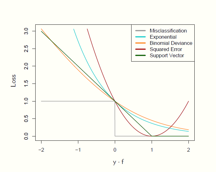
Which of these might work best may be specific to the situation, but the gist is that they penalize negative values (misclassifications) more heavily and increasingly (except for misclassification error, which penalizes all misclassifications equally), with their primary difference in how heavy that penalty is.

Regularization

It is important to note that a model fit to a single data set might do very well with the data at hand, but then suffer when predicting independent data¹³. Also, oftentimes we are interested in a ‘best’ subset of predictors among a great many, and in this scenario the estimated coefficients are overly optimistic. This general issue can be improved by shrinking estimates toward zero, such that some of the performance in the initial fit is sacrificed for improvement with regard to prediction.

Penalized estimation will provide estimates with some shrinkage, and we can use it with little additional effort with our common procedures. Concretely, let’s apply this to the standard linear model, where we are finding estimates of \(\beta\) that minimize the squared error loss.

\[\hat\beta = \underset{\beta}{\mathrm{arg\, min}} \sum{(y-X\beta)^2}\]

In words, we’re finding the coefficients that minimize the sum of the squared residuals. Now we just add a penalty component to the procedure as follows.

\[\hat\beta = \underset{\beta}{\mathrm{arg\, min}} \sum{(y-X\beta)^2} + \lambda\overset{p}{\underset{j=1}{\sum}}{\left|\beta_j\right|}\]

In the above equation, \(\lambda\) is our penalty term¹⁴ for which larger values will result in more shrinkage. It’s applied to the \(L_1\) or Manhattan norm of the coefficients, \(\beta_1,\beta_2...\beta_p\), i.e. not including the intercept \(\beta_0\), and is the sum of their absolute values (commonly referred to as the lasso¹⁵). For generalized linear and additive models, we can conceptually express a penalized likelihood as follows:

\[l_p(\beta) = l(\beta) - \lambda\overset{p}{\underset{j=1}{\sum}}{\left|\beta_j\right|}\]

As we are maximizing the likelihood, the penalty is a subtraction, but nothing inherently different is shown. If we are minimizing the negative (log) likelihood, we then add the penalty. This basic idea of adding a penalty term will be applied to all machine learning approaches, but as shown, we can apply such a tool to classical methods to boost prediction performance.

It should be noted that we can go about the regularization in different ways. For example, using the squared \(L_2\) norm results in what is called (a.k.a. Tikhonov regularization)¹⁶, and using a weighted combination of the lasso and ridge penalties gives us elastic net regularization. We’ll see an example of this later.

R Example

In the following example, we take a look at the lasso approach for a standard linear model. We add the regularization component, with a fixed penalty \(\lambda\) for demonstration purposes¹⁷. However, you should insert your own values for \(\lambda\) in the optim line to see how the results are affected. I’ve also increased the number of predictors to 10.

# data setup
set.seed(123)
N = 100
X = cbind(1, matrix(rnorm(N*10), ncol=10))
beta = runif(ncol(X))
y =  rnorm(N, X%*%beta, sd=2)

sqerrloss_reg = function(beta, X, y, lambda=.5){
  mu = X%*%beta
  # sum((y-mu)^2) + lambda*sum(abs(beta[-1])) # conceptual
  sum((y-mu)^2) + 2*length(y)*lambda*sum(abs(beta[-1])) # actual for lasso
}

lm_result = lm(y~., data.frame(X[,-1]) )
regularized_result = optim(par=rep(0, ncol(X)), 
                           fn=sqerrloss_reg, 
                           X=X, 
                           y=y, 
                           method='BFGS')

From the above, we can see in this case that the penalized coefficients have indeed shrunk toward zero. Now we move to testing. Normally both the training and test sets will be a random split of the original set, for this demo we’ll generate the test as we did with the training.

# Create test data
N_test = 50
X_test = cbind(1, matrix(rnorm(N_test*10), ncol=10))
y_test = rnorm(N_test, X_test%*%beta, sd=2)

# fits on training set
fits_lm = fitted(lm_result, newdata = data.frame(X))
fits_reg = X%*%regularized_result$par

# loss on training set
data.frame(lm_train = crossprod(y - fits_lm),
           regularized_train = crossprod(y - fits_reg))

  lm_train regularized_train
1 402.2046          583.3891

# fits on test set
fits_lm = predict(lm_result, newdata = data.frame(X_test))
fits_reg = X_test%*%regularized_result$par

# loss on test set
data.frame(lm_test = crossprod(y_test - fits_lm),
           regularized_test = crossprod(y_test - fits_reg))

   lm_test regularized_test
1 254.0681         232.4942

We can see that the residual sum of squares has increased just a tad for the regularized fit on the training data. On the test data however, the squared error loss is lower.

In general, we can add the same sort of penalty to any number of models, such as logistic regression, neural net models, recommender systems etc. The primary goal again is to hopefully increase our ability to generalize the selected model to new data. Note that the estimates produced are in fact biased, but we have decreased the variance with new predictions as a counterbalance, and this brings us to the topic of the next section.

Bias-Variance Tradeoff

In most of science, we are concerned with reducing uncertainty in our knowledge of some phenomenon. The more we know about the factors involved or related to some outcome of interest, the better we can predict that outcome upon the influx of new information. The initial step is to take the data at hand, and determine how well a model or set of models fit the data in various fashions. In many applications however, this part is also more or less the end of the game as well¹⁸.

Unfortunately, such an approach, in which we only fit models to one data set, does not give a very good sense of generalization performance, i.e. the performance we would see with new data. While typically not reported, most researchers, if they are spending appropriate time with the data, are actually testing a great many models, among which the ‘best’ is then provided in detail in the end report. Without some generalization performance check however, such performance is overstated when it comes to new data.

In the following, consider a standard linear model scenario, e.g. with squared-error loss function and perhaps some regularization, and a data set in which we split the observations in some random fashion into a training set, for initial model fit, and a test set, which will be kept separate and independent, and used to measure generalization performance¹⁹. We note training error as the (average) loss over the training set, and test error as the (average) prediction error obtained when a model resulting from the training data is fit to the test data. So, in addition to the previously noted goal of finding the ‘best’ model (model selection), we are interested further in estimating the prediction error with new data (model performance).

Bias & Variance

We start²⁰ with a true data generating process for some target \(y\), expressed as a function of features \(X\). We can specify the true model as

\[y = f(X) + \epsilon\]

where \(f(x)\) is the expected value of \(y\) given \(X\), i.e. \(f(x) = E(y|X)\). The expected value of the error, \(E(\epsilon)=0\), has some variance, \(\textrm{Var}(\epsilon) = \sigma^2_\epsilon\). In other words, we are talking about the standard regression model we all know and love. Now we can conceptually think of the expected prediction error at a specific input \(X = x_*\) as:

\[\text{Error}_{x_*} = \text{Irreducible Error} + \text{Bias}^2 + \text{Variance}\]

To better understand this, think of training models over and over, each time with new training data, but testing each model at input \(x_*\). The \(\text{Error}_{x_*}\) is the average, or expected value of the prediction error in this scenario, or \(E[(y - \hat f(x))^2|X=x_*]\), with \(\hat f\) our current estimate of the true underlying data generating function \(f\). We can note three components to this general notion of prediction error:

Irreducible error: The variance of the (new test) target (\(\sigma^2_\epsilon\)). This is unavoidable, since our \(y\) is measured with error.

Bias²: the amount the average of our estimate varies from the true (but unknown) value (\(E(\hat f) - f\)). This is often the result of trying to model the complexity of nature with something much simpler that the human brain can understand. While the simpler might make us feel good, it may not work very well.

Variance: the amount by which our prediction would change if we had estimated it using a different training data set (\(Var(\hat f)\)). Even with unbiased estimates, we could still see a high mean squared error due to high variance.

Slightly more formally, we can present this as follows, with \(h_*\) our estimated (hypothesized) value at \(x_*\):

\[\text{Error}_{x_*} = \text{Var}(\epsilon) + (\text{E}[h_*] - f(x_*))^2 + \text{Var}(h_*)\]

The latter two components make up the mean squared error in our previous demonstration. While they are under our control, they compete with one another such that oftentimes we improve one at the detriment of the other. In other words, bias and variance are not independent.

The Tradeoff

Outlining a general procedure, we start by noting the prediction error on a training data set with multiple models of varying complexity (e.g. increasing the number of predictor variables, adding polynomial terms, including interactions), and then assess the performance of the chosen models in terms of prediction error on the test set. We then perform the same activity for a total of 100 simulated data sets, for each level of complexity.

The results from this process might look like the following, taken from Hastie, Tibshirani, and Friedman (2009). With regard to the training data, we have \(\mathrm{error}_{\mathrm{train}}\) for one hundred training sets for each level of model complexity. The bold blue line notes this average error over the 100 sets by model complexity, and we can see that more complex models fit the data better. The bold red line is the average test error (\(\mathrm{error}_{\mathrm{test}}\)) across the 100 test data sets, and it tells a different story. When models get too complex, the test error starts to increase.

Ideally we’d like to see low bias and (relatively) low variance, but things are not so easy. One thing we can see clearly is that \(\mathrm{error}_{\mathrm{train}}\) is not a good estimate of \(\mathrm{error}_{\mathrm{test}}\), which is now our focus in terms of performance. If we think of the training error as what we would see in typical research where one does everything with a single data set, we are using the same data set to fit the model and assess error. As the model is adapted to that data set specifically, it will be overly optimistic in the estimate of the error, that optimism being the difference between the error rate we see based on the training data versus the average of what we would get with many test data sets. We can think of this as a problem of overfitting to the training data. Models that do not incorporate any regularization or validation process of any kind are likely overfit to the data presented.

Generally speaking, the more complex the model, the lower the bias, but the higher the variance, as depicted in the graphic. Specifically however, the situation is more nuanced, where the type of problem (classification with 0-1 loss vs. continuous response with squared error loss²¹) and technique (a standard linear model vs. regularized fit) will exhibit different bias-variance relationships.

Diagnosing Bias-Variance Issues & Possible Solutions

The following can serve as a visual summary of the concepts just outlined (figure adapted from Domingos (2012)).

Now let’s assume a regularized linear model with a standard data split into training and test sets. We will describe different scenarios with possible solutions.

Worst Case Scenario

Starting with the worst case scenario, poor models may exhibit high bias and high variance. One thing that will not help this situation (perhaps contrary to intuition) is adding more data. You can’t make a silk purse out of a sow’s ear (usually), and adding more data just gives you a more accurate picture of how awful your model is. One might need to rework the model, e.g. adding new predictors or creating them via interaction terms, polynomials, or other smooth functions as in additive models, or simply collecting better and/or more relevant data.

High Variance

When variance is a problem, our training error is low while test error is relatively high (overfitting problem). Implementing more shrinkage or other penalization to model complexity may help with the issue. In this case more data may help as well.

High Bias

With bias issues, our training error is high and test error is not too different from training error (underfitting problem). Adding new predictors/features, e.g. interaction terms, polynomials etc., can help here. Additionally, reducing the penalty parameter \(\lambda\) would also work with even less effort, though generally it should be estimated rather than explicitly set.

Here is another visualization to drive the point home.

The figure is inspired by Murphy (2012) (figure 6.5) showing the bias-variance trade-off. Sample (left) and average (right) fits of linear regression using a Gaussian radial basis function expansion. The blue line represents the true x-y relationship. The top row shows low variance between one fit and the next (left) but notable bias (right) in that the average fit is off. Compare to the less regularized (high variance, low bias) situation of the bottom row. See the kernlab package for the fitting function used, and the appendix for the code used to produce the graph.

Bias-Variance Summary

One of the key ideas any applied researcher can take from machine learning concerns the bias-variance trade-off and issues of overfitting in particular. Typical applied practice involves potentially dozens of models fit to the same data set without any validation whatsoever, yet only one or two are actually presented in publication. Many disciplines report nothing but the statistical significance, and yet one can have statistically significant predictors and have predictive capability that is no different from guessing. Furthermore, very complex models are often fit to small data sets, compounding the problem.

It is very easy to describe science without ever talking about statistical significance. It is impossible to talk about science without talking about prediction. The bias-variance trade-off is one way to bring the concerns of prediction to the forefront, and any applied researcher can benefit from thinking about its implications²².

Cross-Validation

As noted in the previous section, in machine learning approaches we are particularly concerned with prediction error on new data. The simplest validation approach would be to split the data available into a training and test set as discussed previously. We estimate the model on the training data, and apply the model to the test data, get the predictions and measure our test error, selecting whichever model results in the least test error. The following displays a hypothetical learning curve from the results of such a process. While the approach is fairly simple, other approaches are more commonly used and result in better estimates of predictive performance²³.

Adding Another Validation Set

One technique that might be utilized for larger data sets, is to split the data into training, validation, and test sets. For example, one might take the original data and create something like a 60-20-20% split to create the needed data sets. The purpose of the initial validation set is to select the optimal model and determine the values of tuning parameters. These are parameters which generally deal with how complex a model one will allow, but for which one would have little inkling as to what they should be set at beforehand. For example, our \(\lambda\) shrinkage parameter in regularized regression would be such a parameter. We first select models/tuning parameters that minimize the validation set error, and once the model is chosen, we then examine test set error performance. In this way performance assessment is still independent of the model development process.

K-fold Cross-Validation

In many cases we don’t have enough data for such a split, and the split percentages are arbitrary anyway, with results that would be specific to the split chosen. Instead we can take a typical data set and randomly split it into \(\kappa=10\) equal-sized (or close to it) parts. Next, we take the first nine partitions, combine them, and use them as the training set. With chosen model from the training data, make predictions on the held-out partition. Now we do it again, but this time use the 9^th partition as the holdout set. Repeat the process until each of the initial 10 partitions of data have been used as the test set. Average the error across all procedures for our estimate of prediction error. With enough data, this (and the following methods) could be used as the validation procedure before eventual performance assessment on an independent test set with the final chosen model.

An illustration of 3-fold classification.

Leave-one-out Cross-Validation

Leave-one-out (LOO) cross-validation is the same thing but where \(\kappa=N\). In other words, we train a model for all observations except the \(\kappa^{th}\) one, assessing fit on the observation that was left out. We then cycle through until all observations have been left out once to obtain an average accuracy.

Of the two, K-fold may have relatively higher bias but less variance, while LOO would have the converse problem, as well as possible computational issues²⁴. K-fold’s additional bias would be diminished would with increasing sample sizes, and generally 5 or 10-fold cross-validation is recommended. However, many model selection techniques (e.g. via AIC) have a leave-one-out interpretation.

Bootstrap

With a bootstrap approach, we draw \(B\) random samples with replacement from our original data set, creating \(B\) bootstrapped data sets of the same size as the original data. We use the \(B\) data sets as training sets and, using the original data as the test set, average the prediction error across the models.

Other Stuff

Along with the above there are variations such as repeated cross validation, the ‘.632’ bootstrap and so forth. One would want to do a bit of investigating, but \(\kappa\)-fold and bootstrap approaches generally perform well. If variable selection is part of the goal, one should be selecting subsets of predictors as part of the cross-validation process, not at some initial data step.

References

Hastie, Trevor, Robert Tibshirani, and Jerome Friedman. 2009. The Elements of Statistical Learning: Data Mining, Inference, and Prediction, Second Edition. 2nd ed. 2017. Corr. 12th Printing. Springer.

Domingos, Pedro. 2012. “A Few Useful Things to Know About Machine Learning.” Commun. ACM 55 (10). https://doi.org/10.1145/2347736.2347755.

Murphy, Kevin P. 2012. Machine Learning: A Probabilistic Perspective. The MIT Press.

Well some of you. Many applied methods courses don’t teach the basic maximum likelihood approach, even though it’s the most widely used estimation technique for statistical inference.↩
Type ?optim at the console for more detail.↩
For example, if dealing with probabilities, we technically could use minimize squared errors in the case of classification also. We could use a maximum likelihood for either setting (or minimize the negative log likelihood to turn it into a loss function).↩
In terminology we will discuss further later, such models might have low bias but notable variance.↩
This can be set explicitly or also estimated via a validation approach. As we do not know it beforehand, we can estimate it on a validation data set (not the test set) and then use the estimated value when estimating coefficients via cross-validation with the test set. We will talk more about validation later.↩
See Tibshirani (1996) Regression shrinkage and selection via the lasso.↩
Interestingly, the lasso and ridge regression results can be seen as a Bayesian approach using a zero mean Laplace and Normal prior distribution respectively for the \(\beta_j\).↩
As noted previously, in practice \(\lambda\) would be estimated via some validation procedure.↩
I should note that I do not make any particular claim about the quality of such analysis. In many situations, the cost of data collection is very high, and for all the current enamorment with ‘big’ data, a lot of folks will never have access to big data for their situation (e.g. certain clinical populations). In these situations, getting new data for which one might make predictions is extremely difficult.↩
In typical settings, there are parameters specific to some analytical technique for which one would have no knowledge, and which must be estimated along with the usual parameters of the standard models. The \(\lambda\) penalty parameter in regularized regression is one example of such a tuning parameter. In the best case scenario, we would also have a validation set, where we could determine appropriate values for such parameters based on performance with the validation data set, and then assess generalization performance on the test set when the final model has been chosen. However, methods are available to us in which we can approximate the validation step in other ways.↩
Much of the following is essentially a paraphrase of parts of Hastie, Tibshirani, and Friedman (2009) (chapters 2 and 7).↩
See Friedman (1996) On Bias, Variance, 0/1 Loss and the Curse of Dimensionality for the unusual situations that can arise in dealing with classification error with regard to bias and variance.↩
Note that the bias-variance tradeoff doesn’t readily apply to classification problems, at least not in the same way. To begin, the relationship is multiplicative, and depending on which side of the decision boundary one is on (correct vs. not), it might even be useful to increase the variance. However, if one thinks in terms of predicted probabilities rather than predicted class, one can more or less keep the same mindset.↩
Along with some of the other works cited, see Harrell (2015) for a good discussion of model validation.↩
For squared-error loss situations, there is a Generalized cross-validation (GCV) that can be estimated more directly without actually going to the entire LOO procedure, and functions similarly to AIC.↩