Introduction to R

This introduction to R is very brief and only geared toward providing some basics so that one can understand and run the code associated with the content. It is geared toward an audience that likely has no programming experience whatsoever, but may have had some exposure to traditional statistics packages. If you have some basic familiarity with R you may skip this chapter, though it might serve as a refresher for some.

Getting Started

Installation

As mentioned previously, to begin with R for your own machine, you just need to go to the R website, download it for your operating system, and install. Then go to RStudio, download and install it. From there on you only need RStudio to use R.

Updates occur every few months, and you should update R whenever a new version is released.

Packages

As soon as you install it, R is already the most powerful statistical environment within which to work. However, its real strength comes from the community, which has added thousands of packages that provide additional or enhanced functionality. You will regularly find packages that specifically do something you want, and will need to install them in order to use them.

RStudio provides a Packages tab, but it is usually just as or more efficient to use the install.packages function.

install.packages('mynewfavorite')

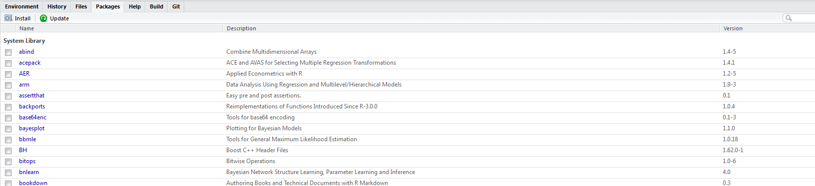
At this point there are over 7000 packages available through standard sources, and many more through unofficial ones. To start getting some ideas of what you want to use, you will want to spend time at places like CRAN Task Views, Rdocumentation, or with a list like this one.

The main thing to note is that if you want to use a package, you have to load it with the library function.

library(lazerhawk)

Sometimes, you only need the package for one thing and there is no reason to keep it loaded, in which case you can use the following approach.

packagename::packagefunction(args)

I suggest using the library function for newbies.

You’ll get the hang of finding, installing, and using packages quite quickly. However, note that the increasing popularity and ease of using R means that packages can vary quite a bit in terms of quality, so you may need to try out a couple packages with seemingly similar functionality to find the best for your situation.

RStudio

RStudio is an integrated development environment (IDE) specifically geared toward R (though it works for other languages too). At the very least it will make your programming far easier and more efficient, at best you can create publish-ready documents, manage projects, create interactive website regarding your research, use version control, and much more. I have an overview here.

See Emacs Speaks Statistics for an alternative. The point is, base R is not an efficient way to use R, and you have at least two very powerful options to make your coding experience easier and more efficient.

Importing Data

It is as easy to import data into R from other programs and text files as it is any other statistical program. As a first step, feel free to use the menu-based approach via the Environment tab.

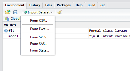
Note that you have easy access to the code that actually does the job. You should quickly get used to a code-based approach as soon as possible, that way you don’t waste time clicking and hunting for files, and instead can quickly run a single line of code. It is easier to select specific options as well. Some key packages to note:

base: Base R already can read in tab-delimited, comma-separated etc. text files
foreign: Base R comes with the foreign package that can read in files from other statistical packages. However support for Stata ended with version 12.

Newer packages

readr: enhanced versions of Base R read functionality
haven: replacement for foreign that can also read current Stata files
readxl: for Excel specifically

There are many other packages that would be of use for special situations and other less common file types and structures.

Key things to know about R

R is a programming language, not a ‘stats package’

The first thing to note for those new to R is that R is a language that is oriented toward, but not specific to, dealing with statistics. This means it’s highly flexible, but does take some getting used to. If you go in with a spreadsheet style mindset, you’ll have difficulty, as well as miss out on the power it has to offer.

Never ask if R can do what you want. It can.

The only limitation to R is the user’s programming sophistication. The better you get at statistical programming the further you can explore your data and take your research. This holds for any statistical endeavor whether using R or not.

Main components: script, console, graphics device

With R, the script is where you write your R code. While you could do everything at the console, this would be difficult at best and unreproducible. The console is where the results are produced from running the script. Again you can do one-liner stuff there, such as getting help for a function. The graphics device is where visualizations are produced, and in RStudio you have two, one for static plots, and a viewer for potentially interactive ones.

R is easy to use, but difficult to master.

If you only want to use R in an applied fashion, as we will do here, R can be very easy to use. As an example the following code would read in data and run a standard linear regression with the lm (i.e. linear model) function.

mydata = read.csv(file='location/myfile.csv')   # some file with an 'x' and 'y' variable
regModel = lm(y ~ x, data=mydata)               # standard regression
summary(regModel)                               # summary of results

The above code demonstrates that R can be as easy to use as anything else, and in my opinion, it is for any standard analysis. In addition, the formula syntax is utilized the vast majority of modeling packages (including lavaan), as is the summary function for printing model results. The nice part is that R can still be easier to use with more complex analyses you either won’t find elsewhere or will only get with crippled functionality.

Object-oriented

This section may be a little more than a newcomer to R wants or even needs to know to get started with R. However, most of the newbie’s errors will be due not knowing a little about this aspect of R programming, and I’ve seen some make the same mistakes even after using R for a long time as a result.

R is object-oriented. For our purposes this means that we create what are called objects and use functions to manipulate those objects in some fashion. In the above code we created two objects, an object that held the data and an object that held the regression results.

Objects can be anything, a character string, a list of 1000 data sets, the results of an analysis, anything.

Assignment

In order to create an object, we must assign something to it. You’ll come across two ways to do this.

myObject = something
myObject <- something

These result in the same thing, an object called myObject that contains ‘something’ in it. For all appropriate practical use, whether you use = or <-is a matter of personal preference. The point is that typical practice in R entails that one assigns something to an object and then uses functions on that object to get something more from it.

Functions

Functions are objects that take input of various kinds and produce some output (simply called a value). In the above code we used three functions: read.csv, lm, and summary. Functions (usually) come with named arguments, that note what types of inputs the function can take. With read.csv, we merely gave it one argument, the file name, but there are actually a couple dozen, each with some default. Type ?read.csv at the console to see the help file.

Classes

All objects have a certain class, which means that some functions will work in certain ways depending on the class. Consider the following code.

x = rnorm(100)
y = x + rnorm(100)
mod = lm(y ~ x)
summary(x)

    Min.  1st Qu.   Median     Mean  3rd Qu.     Max. 
-2.62696 -0.57501  0.13006  0.02673  0.86777  3.20116

summary(mod)


Call:
lm(formula = y ~ x)

Residuals:
     Min       1Q   Median       3Q      Max 
-1.88814 -0.61668  0.01512  0.59158  1.78680 

Coefficients:
            Estimate Std. Error t value Pr(>|t|)    
(Intercept)  0.14936    0.08928   1.673   0.0975 .  
x            1.05172    0.08454  12.440   <2e-16 ***
---
Signif. codes:  0 '***' 0.001 '**' 0.01 '*' 0.05 '.' 0.1 ' ' 1

Residual standard error: 0.8926 on 98 degrees of freedom
Multiple R-squared:  0.6123,    Adjusted R-squared:  0.6083 
F-statistic: 154.7 on 1 and 98 DF,  p-value: < 2.2e-16

In both cases we used the summary function, but get different results. There are two methods for summary at work here: summary.default and summary.lm. Which is used depends on the class of the object given as an argument to the summary function. Most of the time however, there are unique functions that will only work on one class of object.

class(x)

[1] "numeric"

class(mod)

[1] "lm"

One of the most common classes of objects used is the data.frame. Data frames are matrices that contain multiple types of vectors that are the variables and observations of interest. The contents can be numeric, factors (categorical variables), character strings and other types of objects.

nams = c('Bob Ross', 'Bob Marley', 'Bob Odenkirk')
places = c('Dirt', 'Dirt', 'New Mexico')
yod = c(1995, 1981, 2028)

bobs = data.frame(nams, places, yod)
bobs

          nams     places  yod
1     Bob Ross       Dirt 1995
2   Bob Marley       Dirt 1981
3 Bob Odenkirk New Mexico 2028

Case sensitive

A great deal of the errors you will get when you start learning R will result from not typing something correctly. For example, what if we try summary(X)?

summary(X)

Error in summary(X): object 'X' not found

Errors are merely messages or calls for help from R. It can’t do what you ask and needs something else in order to perform the task. In this case, R is telling you it can’t find anything called X, which makes sense because the object name is lowercase \(x\). This error message is somewhat straightforward, but error messages for all programming languages typically aren’t, and depending on what you’re trying to do, it may be fairly vague. If you get an error, your first thought as you start out with R should be to check the names of things.

The lavaan package

You’ll see more later, but in order to use lavaan for structural equation modeling, you’ll need two things primarily: an object that represents the data, and an object that represents the model. It will look something like the following.

modelCode = "
  y ~ x1 + x2 + lv            # structural/regression model
  lv =~ z1 + z2 + z3 + z4     # measurement model with latent variable lv
"

library(lavaan)
mymodel = sem(modelCode, data=mydata)

The character string is our model, and it can actually be kept as a separate file (without the assignment) if desired. Using the lavaan library, we can then use one of its specific functions like cfa, sem, or growth to use the model code object (modelCode above) and the data object (mydata above).

The way to define things in lavaan can be summarized as follows.

formulaType	operator	mnemonic
latent variable definition	=~	is measured by
regression	~	is regressed on
(residual) (co)variance	~~	is correlated with
intercept	~ 1	intercept
fixed parameter	_*	is fixed at the value of _
named parameter	abc*	is named abc

Matching lavaan and R to MPlus

With lavaan and related packages there is almost complete overlap with MPlus. However, there are some things to note.

model	packages
standard CFA, path, SEM, growth	lavaan
missing values	lavaan (FIML), semTools (MI +)
multigroup	lavaan, semTools
mixture models	flexmix, poLCA, many others
Bayesian	blavaan
survey	lavaan, survey.lavaan
multilevel	lavaan (new), mediation
factor score regression	lavaan
visualization	lavaanPlot

The one glaring lack lavaan has regards mixture models, i.e. those with latent categorical variables. However, I’d argue there is far more functionality in R generally, with results that are far more easy to work with than you would have with MPlus. Note that lavaan handles observed categorical variables just fine, though oddly with only a probit link function (no logit).

Up until version 0.6-1 lavaan had no support for multilevel models. However, it now can do two-level SEM, and the mediation package has long been able to do single mediator mixed/multilevel models¹. In addition, lavaan has added some survey support, but you’ll have plenty with survey.lavaan.

Latent variable interactions are not conducted automatically in lavaan. One way to do it is to create a product term for all pairs of items pertaining to two factors, and then specify a latent variable where the manifest variables are the product terms. There is an example provided here, and while the syntax is inefficient, it is conceptually clear.

Unless you have complicated mediation structure (rarely sufficiently justified by SEM practitioners), there is no reason that I can see to do growth curve models. There is far, far more functionality in R for mixed models (e.g. lme4, mgcv, brms), which are the far more common and flexible approach to modeling longitudinal data (and otherwise equivalent). Such models handle nonlinear trends, complicated residual structure, alternative distributions, spatial and phylogenetic correlational structures, and more. MPlus simply doesn’t compete in this realm, and has terribly tedious syntax for either growth curve or multilevel models.

On top of everything else, the lavaan ecosystem, i.e. packages that work with and enhance its models, continues to grow. In addition, with R there are utilities for SEM you won’t find with MPlus, such as model search, regularization, and more. And finally, with the MPlusAutomation package it’s even easier to use MPlus with R than it is to use MPlus itself!

Getting help

Use ? to get the help file for a specific function, or ?? to do a search, possibly on a quoted phrase.

Examples:

?lm
??regression
??'nonlinear regression'

Moving forward

Hopefully you’ll get the hang of things as we run the code in later chapters. You’ll essentially only be asked to tweak code that’s already provided. This document (and associated workshop) is not the place to learn R. However, here are some exercises to make sure we start to get comfortable with it.

Exercises

Interactive version here

Create an object that consists of the numbers one through five. using c(1,2,3,4,5) or 1:5
Create a different object, that is the same as that object, but plus 1 (i.e. the numbers two through six).
Without creating an object, use cbind and rbind, feeding the objects you just created as arguments. For example cbind(obj1, obj2).
Create a new object using data.frame just as you did rbind or cbind in #3.
Inspect the class of the object, and use the summary function on it.

Summary

There’s a lot to learn with R, and the more time you spend with R the easier your research process will likely go, and the more you will learn about statistical analysis.

In practice, these models are problematic even for MPlus.↩