Standard Documents
R Markdown files
R Markdown files, with extension *.Rmd, are a combination of text, R code, and possibly other code or syntax, all within a single file. Various packages, e.g. rmarkdown, knitr, pandoc, etc., work behind the scenes to knit all those pieces into one coherent whole, in whatever format is desired67. The knitr package is the driving force behind most of what is done to create the final product.
HTML
I personally do everything in HTML because it’s the most flexible, and easiest to get things looking the way you want. Presumably at some point, these will simply be the default that people both use and expect in the academic realm and beyond, as there is little additional value that one can get with PDF or MS Word, and often notably less. Furthermore, academia is an anachronism. How much do you engage PDF and Word for anything else relative to how much you make use of HTML (i.e. the web)?
Text
Writing text in a R Markdown document is the same as anywhere else. There are a couple things you’ll use frequently though.
- Headings/Subheadings: Specified #, ##, ### etc.
- Italics & bold: *word* for italics **word** for bold. You can also use underscores (some Markdown flavors may require it).
- Links:
[some_text](http://webaddress.com) - Image:
 - Lists: Start with a dash or number, and make sure the first element is separated from any preceding text by a full blank line. Then separate each element by a line.
Some *text*.

- List item 1
- List item 2

1. item #1
2. item #2
That will pretty much cover most of your basic text needs. For those that know HTML & CSS, you can use those throughout the text as you desire as well. For example, sometimes I need some extra space after a plot and will put in a <br>.
Code
Chunks
After text, the most common thing you’ll have is code. The code resides in a chunk, and looks like this. You can add it to your document with the Insert menu in the upper right of your Rmd file, but as you’ll be needing to do this all the time, instead you’ll want to use the keyboard shortcut of Ctrl/Cmd + Alt/Option + I68.
```{r}
x = rnorm(10)
```
There is no limit to what you put in an R chunk. I don’t recommend it, but it could be hundreds of lines of code! You can put these anywhere within the document. Other languages, e.g. Python, can be used as well, as long as knitr knows where to look for the engine for the code you want to insert69.
Chunk options
There are many things to specify for a specific chunk, or to apply to all chunks. The example demonstrates some of the more common ones you might use.
```{r mylabel, echo = TRUE, eval = TRUE, cache = FALSE, out.width = '50%'}
# code
```
These do the following:
- echo: show the code; can be logical, or line numbers specifying which lines to show
- eval: evaluate the code; can be logical, or line numbers specifying which lines to show
- cache: logical, whether to cache the results for later reuse without reevaluation
- out.width: figure width, can be pixels, percentage, etc.
You can also specify these as defaults for the whole document by using a chunk near the beginning that looks something like this.
```{r setup}
knitr::opts_chunk$set(
  echo = T,
  message = F,
  warning = F,
  error = F,
  comment = NA,
  R.options = list(width = 220),
  dev.args = list(bg = 'transparent')
)
```
There are quite a few options, so familiarize yourself with what’s available, even if you don’t plan on using it, because you never know.
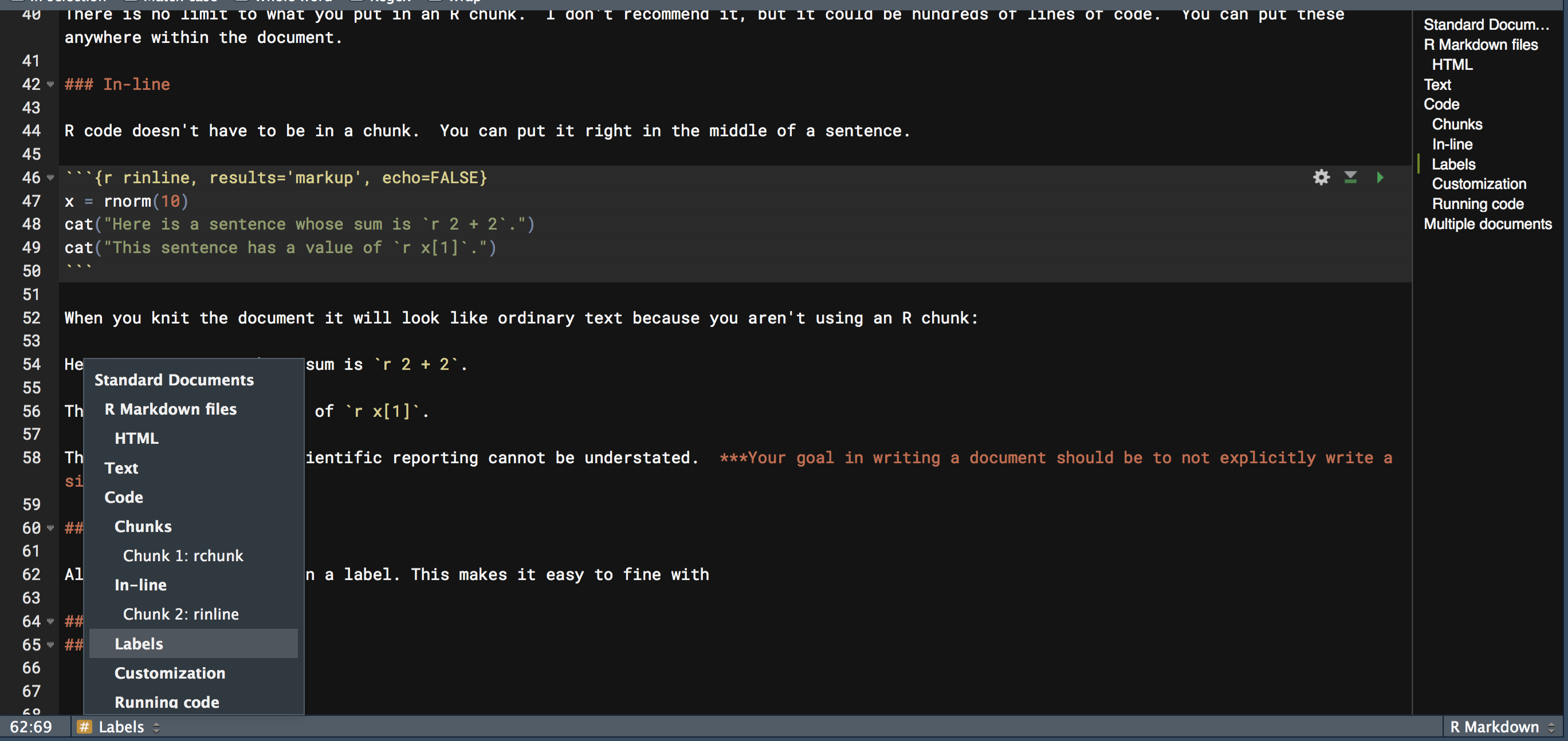
In-line
R code doesn’t have to be in a chunk. You can put it right in the middle of a sentence.
Here is a sentence whose sum is `r 2 + 2`.This sentence has a value of `r x[1]`.When you knit the document, it will look like ordinary text because you aren’t using an R chunk:
Here is a sentence whose sum is 4.
This sentence has a value of 1.955294.
This effect of this in scientific reporting cannot be understated.
Your goal in writing a document should be to not explicitly write a single number that’s based on data.
Labels
All chunks should be given a label. This makes it easy to find it within your document because there are two outlines available to you. One that shows your text headers (to the right), and one that you can click to reveal that will also show your chunks (bottom left). If they just say Chunk 1, Chunk 2 etc., it doesn’t help you to know what they’re doing. There is also some potential benefit in terms of caching, which we’ll discuss later.
Running code
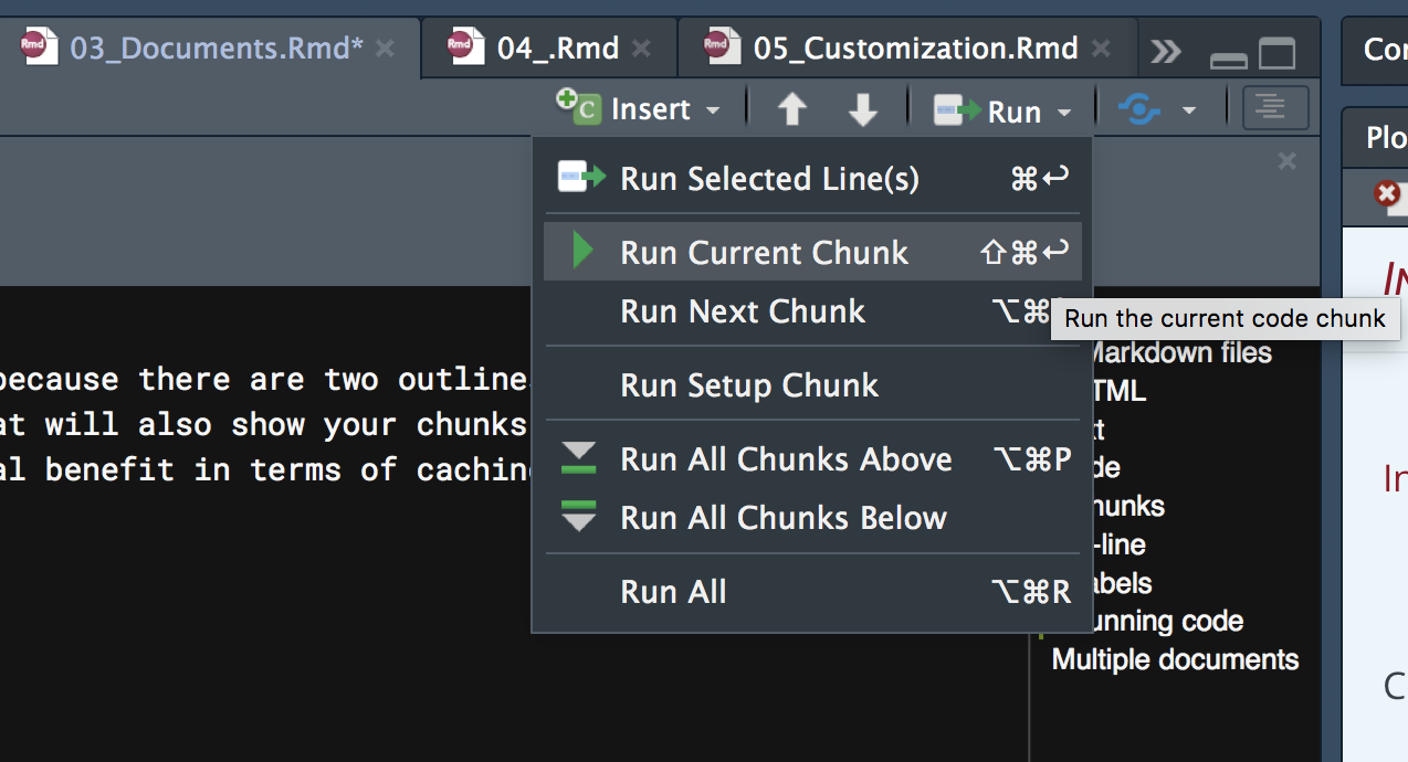
You don’t have to knit the document to run the code, and often you’ll be using the results as you write the document. You can run a single chunk or multiple chunks. Use the shortcuts instead of the menu.
By default, when you knit the document, all code will be run. Depending on a variety of factors, this may or may not be what you want to do, especially if it is time-consuming to do so. We’ll talk about how to deal with this issue in the next part.
Multiple Documents
Knitting multiple documents into one
A single .Rmd file can call others, referred to as child documents, and when you knit that document you’ll have one single document with the content from all of them. You may want to consider other formats, such as bookdown, rather than doing this. Scrolling a lot is sometimes problematic, and not actually required for the presentation of material. It also makes the content take longer to load, because everything has to load70. See the appendix for details.
Parameterized reports
In many cases one may wish to create multiple separate reports that more or less have the same structure. The standard scenario is creating tailored reports, possibly customized for different audiences. In this case you may have a single template which all follow. We can use the YAML configuration to set or load R data objects as follows.
title: institution_name

params:
  institution_name: 'U of M'
  data_folder: 'results/data'
---


``{r}
load(paste0(data_folder, 'myfile.RData'))
``
The result of the above would create a document with the title of ‘U of M’ and load data from the designated data folder. The institution_name and data_folder are processed as R objects before anything else about the document is created.
Parameterized reports combined with child documents mean you can essentially have one document template for all reports as a child template and merely change the YAML configuration for the rest.
Collaboration
R Notebooks are a format one can use that might be more suitable for code collaboration. They are identical to the standard HTML document in most respects, but chunks will by default print output in the Rmd file itself. For example, a graduate student could write up a notebook, and their advisor could then look at the document, change the code as needed etc. Of course, you could just do this with a standard R script as well. Some prefer the inline output however.
For more involved collaborations, I would suggest partitioning the sections into their own document, then use version control keep track of respective contributions, and merge as needed. Such a process was designed for software development, but there’s no reason it wouldn’t work for a document in general, and in my experience, it has quite well.
Using Python for Documents
Most of what we’ve discussed for the standard html document would apply to the Python world as well. The main document format there is the Jupyter Notebook. Like RStudio and R Markdown, Jupyter notebooks seamlessly integrate code and text via markdown, and even can use R instead of Python as well. Jupyter Notebooks are superior to the R Notebook format in most respects, but particularly in look and feel, and interactivity. They are entirely browser-based to use, so whatever you are constructing will look the same if converted to HTML. Almost all the chapters in this document regarding programming, analysis, and visualization have corresponding Jupyter notebooks demonstrating the same thing with Python, including the discussion of notebooks themselves.
Beyond the notebook format, I don’t find it as easy to customize Jupyter notebooks as it is the standard R Markdown HTML document and other formats (e.g. slides, bookdown, interactive web, etc.), which is probably why most of the Jupyter notebooks you come across look exactly the same. With R, one or two clicks in RStudio, or a couple knitr/YAML option adjustments, can make the final product for a basic HTML document look notably different. For Jupyter, one would need various extensions, possibly via the browser, terminal scripting, or would have to directly manipulate html/css. None of this is necessarily a deal-breaker, but most probably would prefer a more straightforward way to change the look.
Pandoc is the universal translator that takes various formats, particularly markup languages, and converts them into others.↩︎
As with RStudio in general, Mac shortcuts for R Markdown documents will deviate from the Windows/Linux ones (in mostly unfortunate/inefficient ways).↩︎
In theory. I’ve had numerous issues trying to use Python via RStudio’s reticulate package, and find it extremely frustrating to use on a Mac (only mildly frustrating on Windows). Other packages, e.g. Stata, cannot pass results from one chunk to the next. When it works, it’s a great resource.↩︎
There is not yet a way within R Markdown that I’m aware of to load on demand as many websites do. However, waiting for things to load until you come to them is annoying at best, and I usually get tired of waiting and move on to other things.↩︎