Plot coefficients for standard linear models.
Source:R/plot_coefficients.lm.R
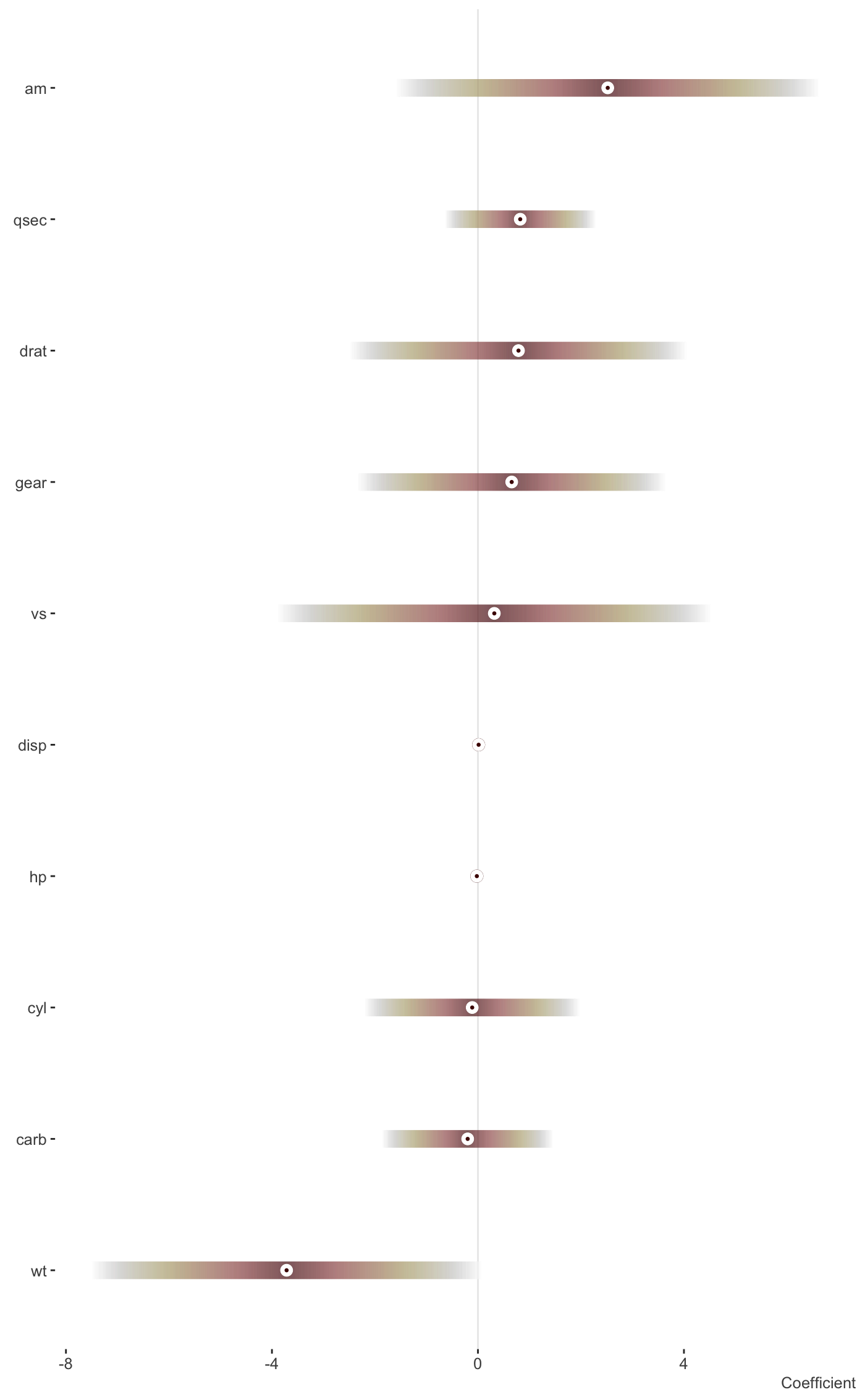
plot_coefficients.lm.RdA basic plot of coefficients with their uncertainty interval for lm and glm objects.
# S3 method for lm
plot_coefficients(
  model,
  order = "decreasing",
  sd_multi = 2,
  keep_intercept = FALSE,
  palette = "bilbao",
  ref_line = 0,
  trans = NULL,
  plot = TRUE,
  ...
)

# S3 method for glm
plot_coefficients(
  model,
  order = "decreasing",
  sd_multi = 2,
  keep_intercept = FALSE,
  palette = "bilbao",
  ref_line = 0,
  trans = NULL,
  plot = TRUE,
  ...
)
Arguments
| model | The lm or glm model |
|---|---|
| order | The order of the plots- "increasing", "decreasing", or a numeric vector giving the order. The default is NULL, i.e. the default ordering. Not applied to random effects. |
| sd_multi | For non-brmsfit objects, the multiplier that determines the width of the interval. Default is 2. |
| keep_intercept | Default is FALSE. Intercepts are typically on a very different scale than covariate effects. |
| palette | A scico palette. Default is 'bilbao'. |
| ref_line | A reference line. Default is zero. |
| trans | A transformation function to be applied to the coefficients (e.g. exponentiation). |
| plot | Default is TRUE, but sometimes you just want the data. |
| ... | Other arguments applied for specific methods. |
Value
A ggplot of the coefficients and their interval estimates. Or the data that would be used to create the plot.
Details
This is more or less a function that serves as the basis for other models I actually use.
See also
Other model visualization:
plot_coefficients.brmsfit(),
plot_coefficients.merMod(),
plot_coefficients(),
plot_gam_2d(),
plot_gam_3d(),
plot_gam_check(),
plot_gam()
Other model visualization:
plot_coefficients.brmsfit(),
plot_coefficients.merMod(),
plot_coefficients(),
plot_gam_2d(),
plot_gam_3d(),
plot_gam_check(),
plot_gam()