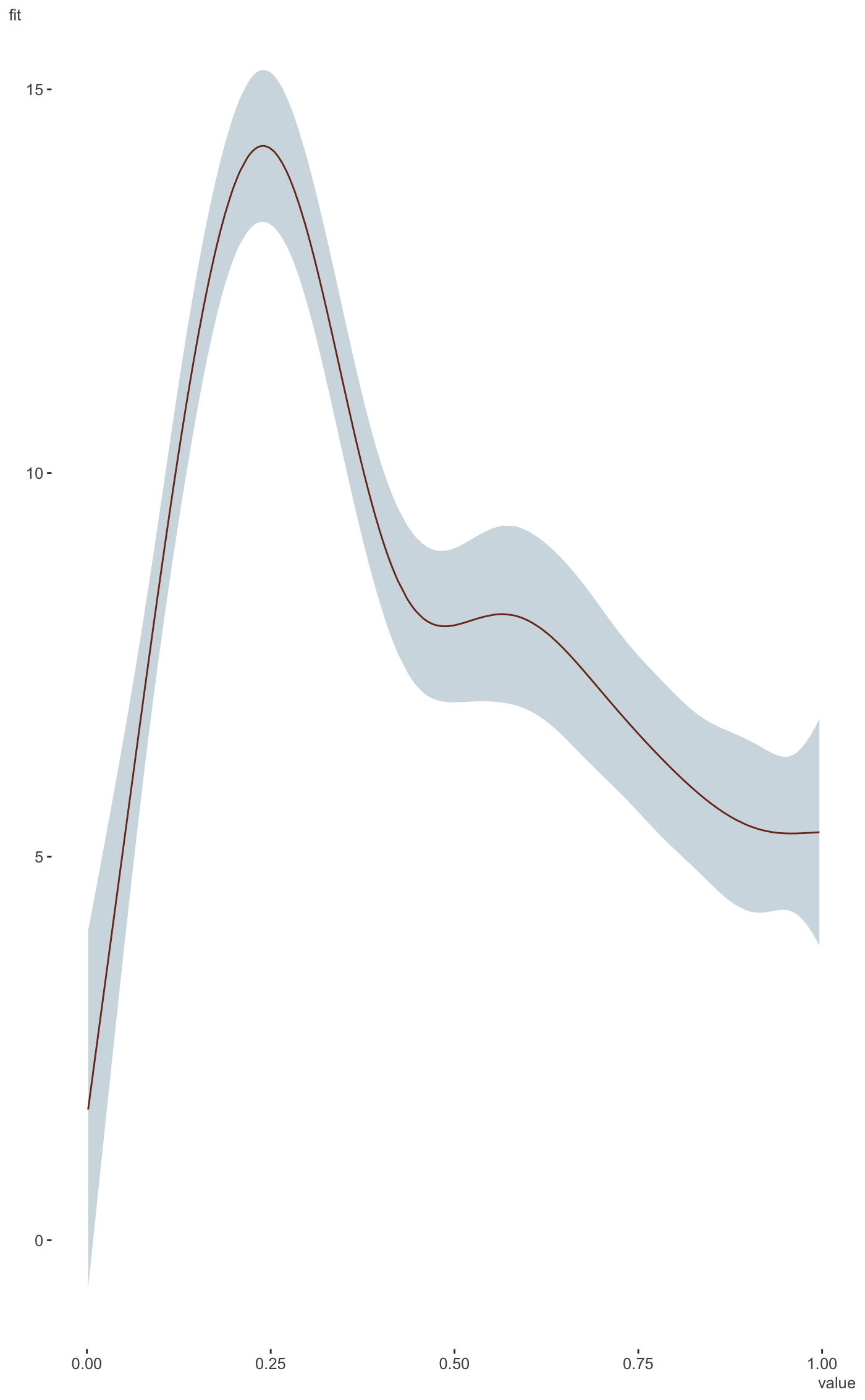
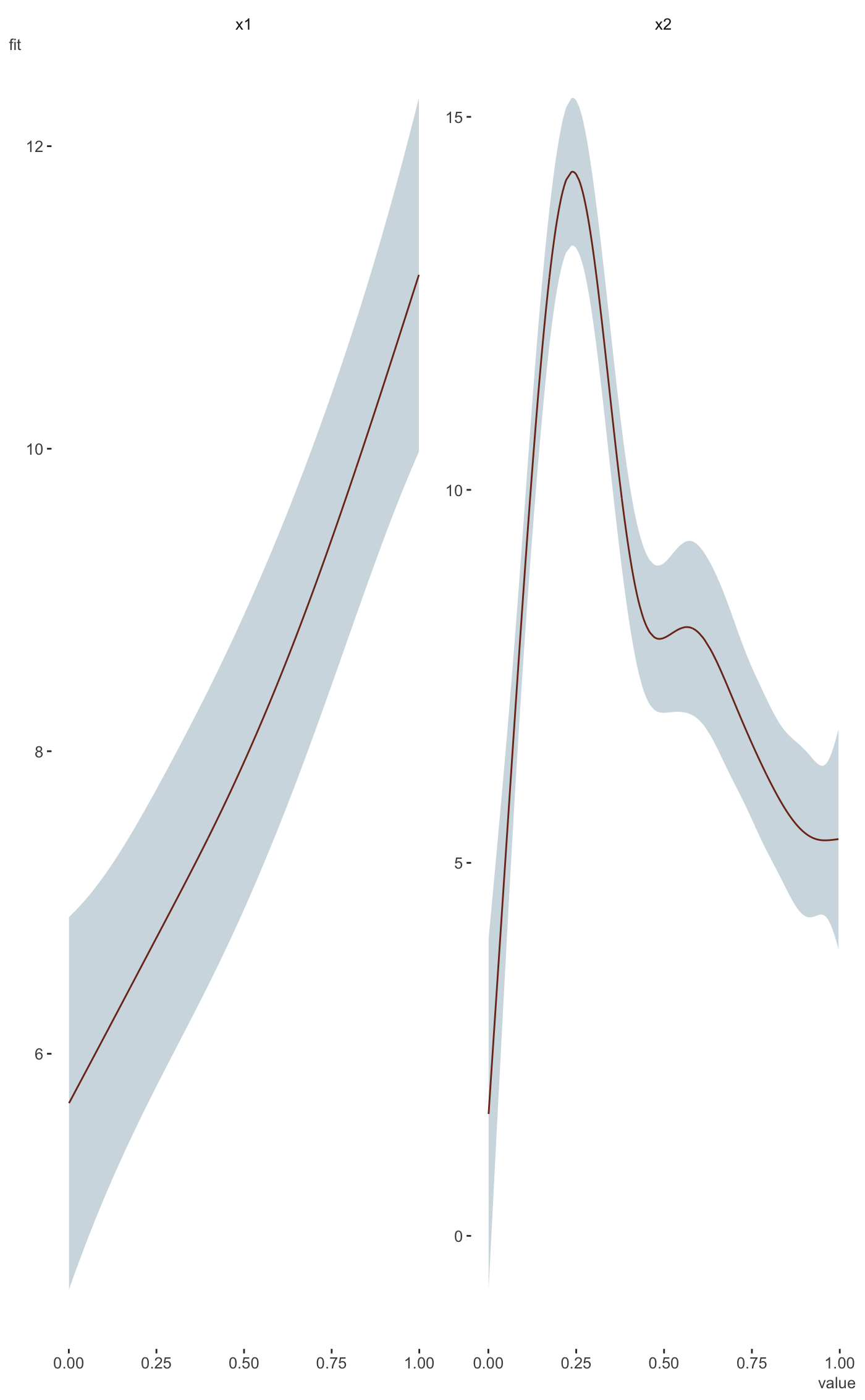
Plot Generalized Additive Model Results

Plot 1d marginal effects from mgcv GAM model results.

plot_gam(
  model,
  main_var,
  conditional_data = NULL,
  line_color = "#7B321C",
  ribbon_color = "#28688640",
  ncol = NULL,
  nrow = NULL
)

plot_gam_1d(
  model,
  main_var,
  conditional_data = NULL,
  line_color = "#ff5500",
  ribbon_color = "#00aaff"
)

plot_gam_multi1d(
  model,
  main_var,
  conditional_data = NULL,
  line_color = "#ff5500",
  ribbon_color = "#00aaff",
  ncol = ncol,
  nrow = nrow
)

Arguments

model	The mgcv GAM.
main_var	Which variable do you want to plot? Uses bare variable names and can take multiple variables via `vars()`.
conditional_data	This is the same as the newdata argument for predict. Supply a data frame with desired values of the model covariates.
line_color	The color of the fitted line.
ribbon_color	The color of the uncertainty interval around the line.
ncol	If plotting multiple smooths, these are passed to facet_wrap.
nrow	If plotting multiple smooths, these are passed to facet_wrap.

Value

a ggplot2 object of the effects of main_var.

Details

This function is fairly 'no-frills' at the moment. Only 1d or multiple 1d smooths of numeric variables are able to be plotted. If conditional data is not supplied, it will be created by create_prediction_data, which defaults to means for numeric, most common category for categorical variables, and 500 observations. It currently will fail if you have a mix of 2d and 1d and do not specify a smooth.

Examples

library(mgcv) # you don't need this function if you don't use this package
#> Loading required package: nlme
#> 
#> Attaching package: ‘nlme’
#> The following object is masked from ‘package:lme4’:
#> 
#>     lmList
#> This is mgcv 1.8-33. For overview type 'help("mgcv-package")'.
library(dplyr)
#> 
#> Attaching package: ‘dplyr’
#> The following object is masked from ‘package:nlme’:
#> 
#>     collapse
#> The following objects are masked from ‘package:stats’:
#> 
#>     filter, lag
#> The following objects are masked from ‘package:base’:
#> 
#>     intersect, setdiff, setequal, union
# example taken from the mgcv plot.gam help file.
set.seed(0)
## fake some data...
f1 <- function(x) {
  exp(2 * x)
}
f2 <- function(x) {
  0.2 * x ^ 11 * (10 * (1 - x)) ^ 6 + 10 * (10 * x) ^ 3 * (1 - x) ^ 10
}
f3 <- function(x) {
  x * 0
}

n <- 200
sig2 <- 4

d = tibble(
  x0 = rep(1:4, 50),
  x1 = runif(n, 0, 1),
  x2 = runif(n, 0, 1),
  x3 = runif(n, 0, 1),
  e  = rnorm(n, 0, sqrt(sig2)),
  y  = 2 * x0 + f1(x1) + f2(x2) + f3(x3) + e
) %>%
  mutate(x0 = factor(x0))

b <- gam(y ~ x0 + s(x1) + s(x2) + s(x3), data = d)

library(visibly)

plot_gam(b,
         conditional_data = tibble(x2 = runif(500)),
         main_var = x2)

plot_gam(b, main_var = x2)


plot_gam(b, main_var = vars(x2, x1))

plot_gam(b,
         conditional_data = tibble(x1 = runif(500),
                                       x2 = runif(500)),
         main_var = vars(x2, x1))

# compare with mgcv plot
plot(b, pages=1)

Plot Generalized Additive Model Results

Arguments

Value

Details

See also

Examples